May
24
2017
 If you're like me and have had to merge spreadsheets of club members with training records whilst looking up values from another spreadsheet, then you've probably come across VLOOKUP, and you probably went a bit mad. VLOOKUP works great in limited slices, but it has some serious limitations. Like only matching on one column, and needing your sheet to be sorted by the match field. For me it was always a frustrating, risky activity that had me reaching for the Whiskey bottle.
Well, I've found a solution. It's a bit harder to set up but it's way better than VLOOKUP and gives you rock solid matches on multiple columns.
Read on, your life will never be the same.
The Setup

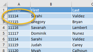
Diagram 1: The SourceData Table. In this example we're going to match the Username and the Start Date.

Diagram 2: The ResultsData Sheet. Column G and H go and lookup values in the SourceData sheet.
You can download the sample sheet here
I've found this method simpler if you have one workbook with two worksheets in it: one for the source data with what you're looking for, and one that will get the results of the matching data. In my sample spreadsheet they're called 'SourceData' and 'ResultsData'. You might have to do some cutting and pasting but I assume you can do that just fine. There are two extra things that you'll find helpful:
- When you edit a formula using this method then instead of hitting 'Enter' to update the formula, hit 'CTRL' + 'SHIFT' + 'ENTER'. The formula gets saved as an 'Array Formula'. Look that up if you want but basically just remember that any time you edit the formula you have to save it with 'CTRL' + 'SHIFT' + 'ENTER'.
- If you want to lock a formula to a set range then you can make it Absolute by adding $ signs to the values in the cell range. So, A1:C3 can get messed up when a cell is dragged around to copy it to another cell, but if you write it as $A$1:$C$3 then it will always be that cell range. You can even combine this and have just part of the range set as Absolute, for example, $A1:C$3.
So the magic formula
Here it is:
=INDEX(SourceData!$A$1:$I$16,MATCH(A3&F3,SourceData!A:A&SourceData!F:F,0),8)
The important stuff is colour coded. Let's break it down. The MATCH command says "Find me this" and the cool thing about Arrays is that you can tell it to match on more than one cell.
So, in the green A3&F3 you can see it saying match the UserID and the Start Date. The cool thing is that you can add three or four or five match criteria.
The red part of the formula specifies the columns to look in for the matched values SourceData!A:A&SourceData!F:F Basically, Column A for the Username and Column F for the Start date.
And then, SourceData!$A$1:$I$16 says where to go and look for a match.
Finally, the last little bit in pink SourceData!F:F,0),8) which says what column value do you want me to return? In this case the eighth column.
The little trick to remember is that when you save this formula you have to hit 'CTRL' + 'SHIFT' + 'ENTER' to save it as an array. You'll know it has been saved as an Array because the formula will have {} around it. for example {=INDEX(SourceData!$A$1:$I$16,MATCH(A3&F3,SourceData!A:A&SourceData!F:F,0),8)} Don;t worry if you loose these brackets, the cell will just get #N/A in it and you can reedit the cell and Save with 'CTRL' + 'SHIFT' + 'ENTER'.
Some little short cuts
- In Excel 01/01/2016 is not the same as 01/01/2016 12:32 PM, even if you format the cell in the Short Date format. So if your stored value includes the time then you will need strip that out. There are many ways to do this, my favourite is =INT(F2) and then format the cell as 'Short Date'. By converting it to an integer you remove the time part which is stored as the decimal part of the whole number.
- Next up is dragging a cell to copy the value or formula down the column or across the row. If you select a cell with a formula you will notice a little square in the bottom right hand corner. If you select that with the mouse and drag down it will copy your value or formula down the column or across the row. If you hold down the control key, it can increments the number or date for you as well. Try it.
- Related to the above is if you double click that little square then it will copy your formula to all cells in a table if it can owrk out if there is a table.
- I mentioned this at the top of the blog, but if you Put $ in fron of row and column reference it means its absolute so they want change if you use the technique above of dragging out a cell. So for example $A$3 rather than A3
- You can use this with one or more columns for matching, you'd just the green and red piece of the formula above, for example A3&F3&G3 and SourceData!A:A&SourceData!F:F&SourceData!G:G or A3&and SourceData!A:A. So easy.
So there you go, this little formula has changed my life, hope it helps you